Creating Word Clouds with Python Libraries

Learn how to create word clouds with the help of WordCloud, Matplotlib, and Pandas libraries.

A word cloud (or tag cloud) is a figure filled with words in different sizes, which represent the frequency or the importance of each word. It’s useful if you want to explore text data or make your report livelier.

Prerequisites

To create a word cloud, we’ll need the following:

Python installed on your machine
Pip: package management system (it comes with Python)
Jupyter Notebook: an online editor for data visualization
Pandas: a library to prepare data for plotting
Matplotlib: a plotting library
WordCloud: a word cloud generator library

You can download the latest version of Python for Windows on the official website.

To get other tools, you’ll need to install recommended Scientific Python Distributions. Type this in your terminal:

    
        
pip install numpy scipy matplotlib ipython jupyter pandas sympy nose wordcloud

Getting Started

Create a folder that will contain your notebook (e.g. “wordcloud”) and open Jupyter Notebook by typing this command in your terminal (don’t forget to change the path):

    
        
cd C:\Users\Shark\Documents\code\wordcloud
py -m notebook

This will automatically open the Jupyter home page at http://localhost:8888/tree. Click on the “New” button in the top right corner, select the Python version installed on your machine, and a notebook will open in a new browser window.

In the first line of the notebook, import all the necessary libraries:

    
        
from wordcloud import WordCloud, STOPWORDS 
import matplotlib.pyplot as plt 
import pandas as pd
%matplotlib notebook

You need the last line — %matplotlib notebook — to display plots in input cells.

Data Preparation

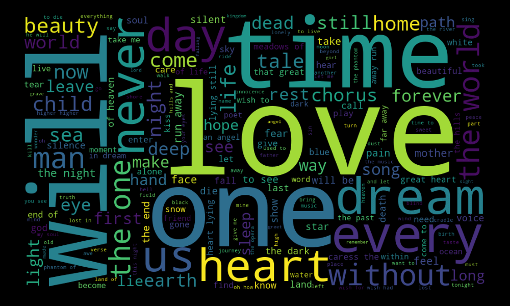
We’ll create a word cloud showing the most commonly used words in Nightwish lyrics, a symphonic metal band from Finland. We’ll create a word cloud from a .csv file, which you can download on Kaggle (nightwish_lyrics.csv).

On the second line in your Jupyter notebook, type this code to read the file:

    
        
df = pd.read_csv('nightwish_lyrics.csv')
df.head()

This will show the first 5 lines of the .csv file:

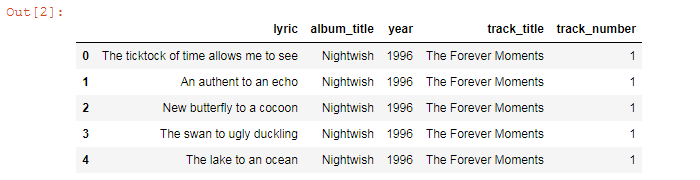
For plotting, we’ll use the first column (data['lyric']) with lines from song lyrics.

Plotting

We’ll create a word cloud in several steps.

1. Set stop words

    
        
comment_words = '' 
stopwords = set(STOPWORDS)
stopwords = ['nan', 'NaN', 'Nan', 'NAN'] + list(STOPWORDS)

The last line is optional. Add NaN values to the stop list if your file or array contains them.

2. Iterate through the .csv file

    
        
values = df['lyric'].values

for val in values: 
    val = str(val) 
    tokens = val.split() 
    for i in range(len(tokens)): 
        tokens[i] = tokens[i].lower() 
    comment_words += ' '.join(tokens)+' '

Here we convert each val (lyric line) to string, split the values (words), and convert each token into a lowercase.

If you’re generating a word cloud not from a .csv file but from a list of words only, you don’t need this part. You can set comment_words and then use the WordCloud() function.

By the way, if you want to get a list of the most frequent words in a text, you can use this Python code:

    
        
text = """...""" # your text

text.split()
count = {}
for word in text.split():
	count.setdefault(word, 0)
	count[word] += 1

list_count = list(count.items())
list_count.sort(key=lambda i: i[1], reverse=True)
for i in list_count:
    print(i[0], ':', i[1])

3. Generate a word cloud

    
        
facecolor = 'black'

wordcloud = WordCloud(width=1000, height=600, 
            background_color=facecolor, 
            stopwords=stopwords,
            min_font_size=10).generate(comment_words)

4. Plot the WordCloud image

    
        
plt.figure(figsize=(10,6), facecolor=facecolor) 
plt.imshow(wordcloud) 
plt.axis('off') 
plt.tight_layout(pad=2)

We’re creating a 1000 × 600 px image so we set figsize=(10,6). This is the size of the figure that can be larger than the word cloud itself. In our code, they’re equal as we previously set WordCloud(width=1000, height=600). In addition, pad=2 allows us to set padding to our figure.

5. Save the chart as an image

    
        
filename = 'wordcloud'
plt.savefig(filename+'.png', facecolor=facecolor)

You might need to repeat facecolor in savefig(). Otherwise, plt.savefig might ignore it.

That’s it, our word cloud is ready. You can download the notebook on GitHub to get the full code.

Popular Tags