In this guide, we’ll do various data manipulations and try out all sorts of Pandas tricks using a Kaggle dataset as an example.
Pandas is a Python library for data manipulation. It works really well when data is in a tabular format and provides objects like DataFrames and Series which are useful for analyzing data.
In this article, we’ll be working with the Super Heroes Dataset that you can download on Kaggle. This dataset is very convenient for learning purposes as it includes different types of data: floating-point numbers, strings, and booleans.
Prerequisites
To start using Pandas, you’ll need to install recommended Scientific Python Distributions. Type this in your terminal:
pip install numpy scipy matplotlib ipython jupyter pandas sympy nose
To import Pandas, simply use this:
import pandas as pd
Reading the file
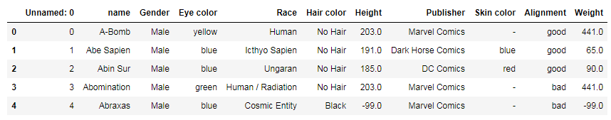
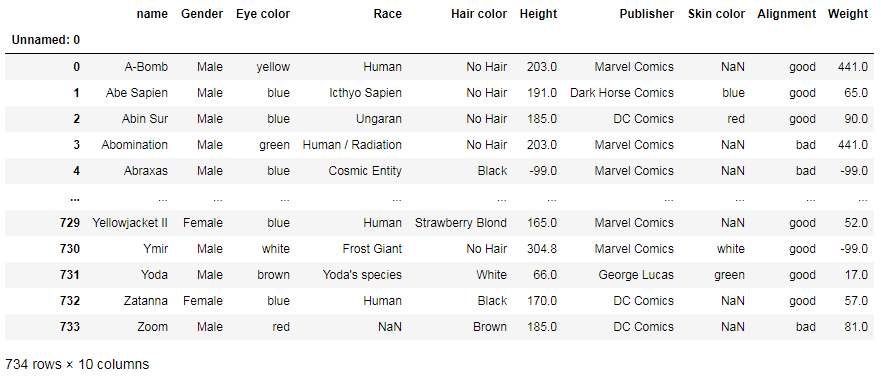
First, let’s read one of the .csv files of the dataset, heroes_information.csv. Here’s the simplest way to do this:
file = 'heroes_information'
df = pd.read_csv(file + '.csv')
df

read_csv has several parameters that are often overlooked:
- names: list of column names
- header: if the file contains a header row, you should pass header=0 to override the column names
- index_col: column to use as the row labels
- usecols: to choose columns you wish to keep
- prefix: prefix to add to column numbers when there’s no header, e.g. 'X' for X0, X1, etc.
- dtype: to specify data types, e.g. {'a': np.float64, 'b': np.int32, 'c': 'Int64'}
- nrows: number of rows to read
- skiprows: number of rows to skip
- na_values: additional strings to recognize as NaN
- skip_blank_lines: True: to skip over blank lines
- parse_dates: parse_dates: True would parse dates in the index, parse_dates: [1, 2, 3] would parse dates in the columns
For example, we can simultaneously read the file, select columns (#0 and #5), rename them, skip the first row (header), and add strings to recognize as NaN:
df = pd.read_csv(file + '.csv',
                 usecols=[0,5], names=['Name', 'Height, cm'],
                 skiprows=1, index_col=0, na_values='-')
Displaying part of the DataFrame
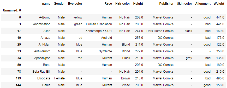
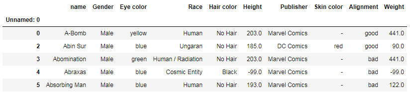
df.head() would display the first 5 rows:
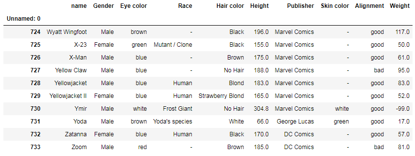
And df.tail() would display the last 5 rows. You can specify the number of rows you want to see:
df.tail(10)
Setting column as index
You can set a column as the index at the same moment when you’re reading the file:
df = pd.read_csv(file + '.csv', index_col=0)
Or you can make a separate command:
df.set_index('Unnamed: 0', inplace=True)
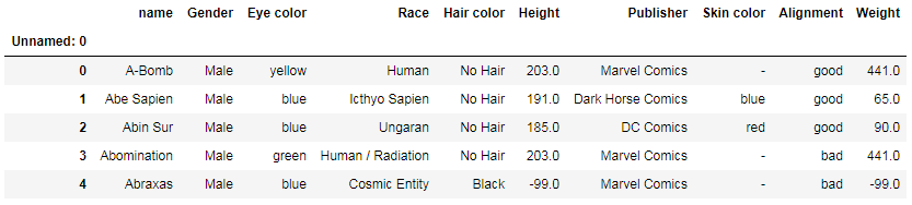
inplace=True modifies the DataFrame in place and doesn’t create a new object.
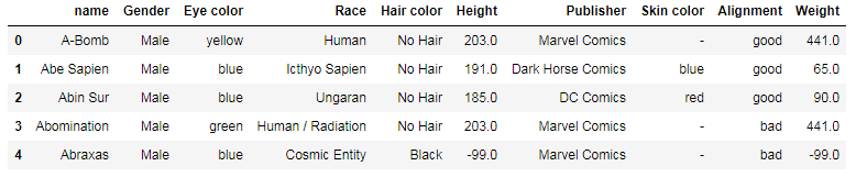
Renaming columns
There are several methods to rename columns:
1. You can set the names parameter when reading the file:
df = pd.read_csv(file + '.csv',
                 usecols=[0,5], names=['Name', 'Height, cm'],
                 skiprows=1, index_col=0, na_values='-')
2. You can explicitly rename columns:
df.rename(columns={
        'name': 'Name',
        'Height': 'Height, cm',
        'Weight': 'Weight, kg'
    }, inplace=True)
Or:
df = df.rename({'name':'Name', 'Height':'Height, cm'}, axis='columns')
3. You can use a string method if you need to rename all of your columns in the same way:
# replace spaces with underscores
df.columns = df.columns.str.replace(' ', '_')

# make lowercase & remove trailing whitespace
df.columns = df.columns.str.lower().str.rstrip()
4. You can overwrite all column names:
df.columns = ['Hero Name', 'Sex', ..., 'Height, cm', ...]
Selecting and deleting columns
Here are some of the lesser-known ways to select columns with Pandas.
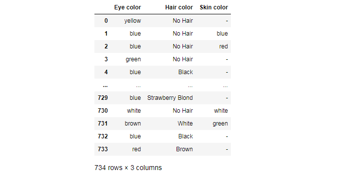
You can select columns by a similar name. For example, you can select only those columns whose names contain the word “color”:
df.filter(like='color', axis=1)
You can also select columns by data type:
df.select_dtypes(include='number')
df.select_dtypes(include=['number', 'category', 'object'])
df.select_dtypes(exclude=['datetime', 'timedelta'])
For example, df.select_dtypes(include='number') would display only those columns that have numeric data.
And if you wish do delete selected columns, you can explicitly enumerate them:
df = df.drop(['Race', 'Publisher', 'Alignment'], axis = 1)
Transposing the table
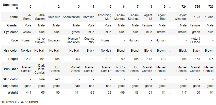
If you want to transpose the index and columns of your table, just use this:
df.T
Selecting values on condition
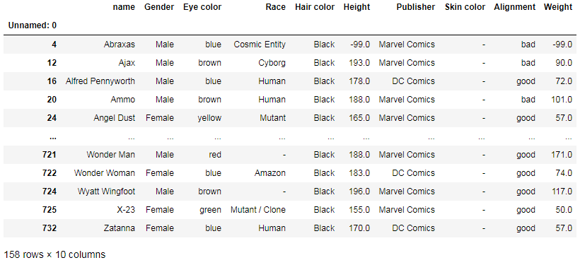
For example, you can select only superheroes with black hair:
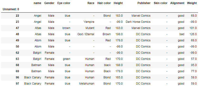
df[df['Hair color'] == 'Black']
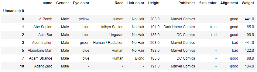
Or you can select superheroes who are taller than 180 cm:
df[df['Height'] >= 180].head(7)
Another way to select all rows with height higher than a specified value:
df[np.abs(df['Height']) > 200]
Or you can select rows with publishers limited to Marvel Comics and DC Comics:
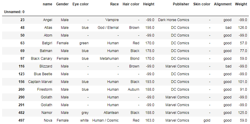
df[(df['Publisher'] == 'Marvel Comics') | (df['Publisher'] == 'DC Comics')].head()
Sorting values
You can sort values using sort_values. For example, if you want to sort superheroes by height from the tallest ones to the shortest ones, you can use this code:
df.sort_values(by='Height', ascending=False)
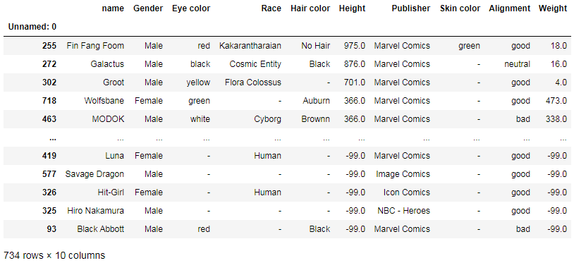
Here we can have a glance at extreme points in superheroes’ heights. This quick sorting shows us that the tallest superhero (975 cm) is Fin Fang Foom and some of the tiniest ones (-99 cm) are Black Abbott, Hiro Nakamura, Hit-Girl, Savage Dragon, and Luna. There may be some issues with the data accuracy, but we’re using this just as an example.
sort_values can have several parameters:
- by: name or list of names to sort by
- axis: 0 or 'index', 1 or 'columns'
- ascending: True or False
- inplace: if True, perform sorting in-place
- na_position: 'first' (puts NaNs at the beginning) or 'last' (puts NaNs at the end)
Binning
If you need to segment and sort data values into bins, use the cut function. First, define bins or intervals to divide your data. Next, apply the cut function. And then, count values for each interval.
heights = df['Height']
bins = [-100, 0, 100, 200, 300, 400, 500, 600, 700, 800, 900]
cats = pd.cut(heights, bins)
cats
Out:

Unnamed: 0
0      (200, 300]
1      (100, 200]
2      (100, 200]
3      (200, 300]
4       (-100, 0]
          ...
729    (100, 200]
730    (300, 400]
731      (0, 100]
732    (100, 200]
733    (100, 200]
Name: Height, Length: 734, dtype: category
Categories (10, interval[int64]): [(-100, 0] < (0, 100] < (100, 200] < (200, 300] ... (500, 600] < (600, 700] < (700, 800] < (800, 900]]
Parenthesis () means an open interval. It doesn’t include values in its endpoints, for example, (0, 1) means “greater than 0 and less than 1”.
And square brackets [] mean a closed interval. It includes values in its endpoints, for example, (0, 1] means “greater than 0 and less or equal to 1”.
pd.value_counts(cats)
Out:

(100, 200]    449
(-100, 0]     217
(200, 300]     51
(0, 100]        9
(300, 400]      5
(800, 900]      1
(700, 800]      1
(600, 700]      0
(500, 600]      0
(400, 500]      0
Name: Height, dtype: int64
Thanks to the binning method, we can learn that most superheroes are between 100 and 200 cm tall, that a significant share is also between -100 and 0 cm tall, and that none is between 400 and 700 cm tall though someone’s height is 700–900 cm.
Retrieving quick stats
The simplest way to retrieve quick stats is using describe(). It automatically selects columns with numeric data and provides a summary of statistical data, such as:
- count: the number of values that are not NaN
- mean: the arithmetic mean, the central value of a set of numbers
- std: standard deviation, a measure of the amount of variation or dispersion of a set of values
- min: the minimum
- 25%: the first quartile
- 50%: the median
- 75%: the third quartile
- max: the maximum
df.describe()

You can also write your own functions to get specific stats that you need. The example below shows how we can get shares of superheroes with specific characteristics:
def get_share(column, value):
    x = len(df[df[column] == value]) / df[column].count() * 100
    return '{:.2f}'.format(x) + '%'

print('Share of female superheroes: ', get_share('Gender', 'Female'))
print('Share of blue-eyed superheroes: ', get_share('Eye color', 'blue'))
print('Share of bad superheroes: ', get_share('Alignment', 'bad'))
Out:

Share of female superheroes:  27.25%
Share of blue-eyed superheroes:  30.65%
Share of bad superheroes:  28.20%
You can also count occurrences of specific words of syllables by using contains(). For example, we can count how often superheroes’ names contain “man”:
df['name'].str.contains('[Mm]an').sum()
Out: 64
Formatting values
Here are some examples showing how we can format values with Python/Pandas.
To format floating numbers with two decimals:
'{:.2f}'.format(x)
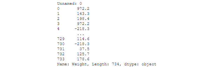
To convert kilograms to pounds (1 kg = 2.20462 lb) in a column:
df['Weight'].map(lambda x: '{:.1f}'.format(x * 2.20462))
To capitalize values:
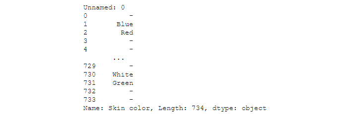
df['Skin color'].str.capitalize()
To select every first word in a string:
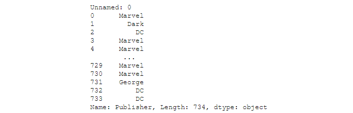
df['Publisher'].str.split().str.get(0)
To select every last word in a string:
df['Publisher'].str.split().str.get(-1)
To convert values to numeric in several columns at once:
df[columns] = df[columns].apply(pd.to_numeric, errors='coerce', axis=1)
Checking uniqueness
There are several ways to check uniqueness of values:
df['name'].is_unique
— Returns True/False.
df['name'].unique()
— Returns a list of unique names.
df[df['name'].duplicated(keep=False)]
— Returns a table with duplicated names, for example:
df[df['name'].duplicated() == True]
— Returns a table with duplicated names only (first-encountered names are omitted), for example:
Handling NaN values
You can replace any values with NaN:
df.replace('-', np.nan)
To replace NaN values with zeros:
df.fillna(0, inplace=True)
To delete all rows with NaN values:
df.dropna(inplace=True)
To drop columns with any missing values:
df.dropna(axis='columns')
To calculate the percentage of missing values in each column:
df.isna().mean()
To drop columns in which more than 10% of values are missing:
df.dropna(thresh=len(df)*0.9, axis='columns')
If you need to fill missing values in time series data, you can use df.interpolate(). You can find more information in Pandas documentation.
Merging several DataFrames
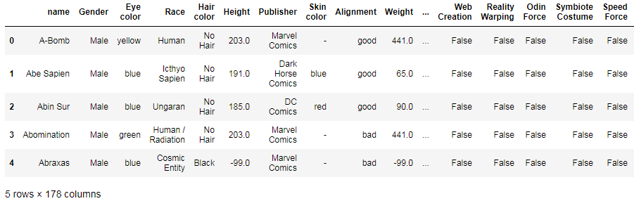
If you need to merge several DataFrames, you can use concat(), for example:
df1 = pd.read_csv('super_hero_powers.csv')
df_m = pd.concat([df, df1], axis=1, ignore_index=False, sort=False, join='outer')
df_m.head()
- axis=1 merges frames horizontally, while axis=0 appends the next DataFrame below the previous one
- ignore_index=True doesn’t duplicate the index
- sort=False doesn’t sort values
- join='outer' merges frames without losing values (includes even empty rows)
Another way is to use merge():
df_merged = pd.merge(df, df1, on='name')
on indicates the key column that is shared by both data frames. Be sure to check whether they have the same column. In our case, the common column is called “name” in the first data frame and “hero_names” in the second one, so we need to rename the first column in our second data frame (super_hero_powers.csv):
df1 = pd.read_csv('super_hero_powers.csv')
df1.rename(columns={'hero_names': 'name'}, inplace=True)
Additionally, if you have multiple files that match the same pattern, you can use glob() to list your files and use a generator expression to read files and concat() to combine them:
from glob import glob
salary_files = sorted(glob('data/salaries*.csv'))
salary_files
Out:
[data/salaries1.csv, data/salaries2.csv, data/salaries3.csv]
pd.concat((pd.read_csv(file) for file in salary_files), ignore_index=True)
Grouping values
To group values and make some operations on them (like mean(), sum(), count(), etc.), use groupby(). This operation involves splitting the object, applying a function, and combining the results.
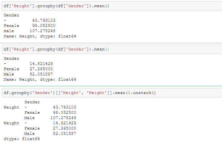
In the examples below, we group values by gender and compute the mean height and weight for each gender:
df['Height'].groupby(df['Gender']).mean()

df['Weight'].groupby(df['Gender']).mean()
You can also apply the groupby operation to several columns at once:
df.groupby('Gender')[['Height', 'Weight']].mean().unstack()
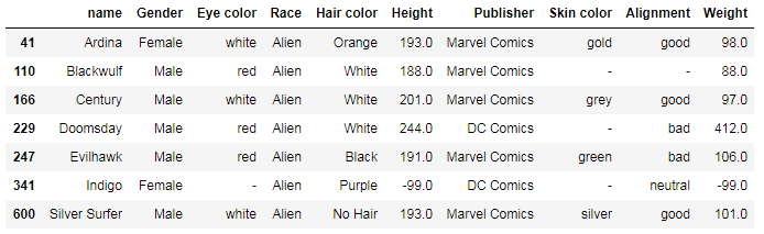
If you've created a groupby object, you can access any of the groups (as a DataFrame) using the get_group() method, for example:
races = df.groupby('Race')
races.get_group('Alien')
Displaying the most common values
With Pandas, you can also get the modes or values that appear most often. Sometimes, this feature allows us to get really interesting insights.
For example, we can group eye-color values by race and get the mode with the aggregate (agg()) function:
df.groupby(['Race'])['Eye color'].agg(pd.Series.mode)

The result shows that, for example, Androids have mostly green eyes and Zombies are generally black-eyed.
Likewise, we can group values related to skin color, hair color, and alignment:
df.groupby(['Race'])['Skin color'].agg(pd.Series.mode).tail(10)

df.groupby(['Race'])['Hair color'].agg(pd.Series.mode).tail(10)

df.groupby(['Race'])['Alignment'].agg(pd.Series.mode)

Or we can group all these values by race at once:
df.groupby(['Race'])[['Eye color', 'Skin color', 'Alignment']].agg(pd.Series.mode)
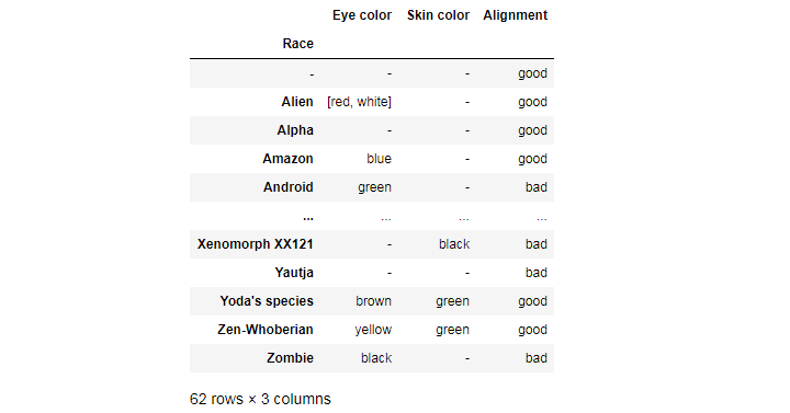
From these, we can conclude that Yoda’s species and Zen-Whoberians are generally green-skinned and good, and that Zombies are mostly black-eyed and bad.
Saving the DataFrame to a .csv file
In the previous example, we created a new valuable DataFrame:
new_df = df.groupby(['Race'])[['Eye color', 'Skin color', 'Alignment']].agg(pd.Series.mode)
If we want to save it to a .csv file, we use the following code:
filename = 'most-common-values'
new_df.to_csv(filename + '.csv')
Visit our Data Visualization section for more articles. Also, don’t forget to follow our profiles on Twitter and Facebook to stay tuned!